Using Postgres and pgRouting To Explore The Smooth Waves of Yacht Rock
pgRouting is a powerful routing tool, usually used for pathfinding/mapping/direction applications. (See Paul Ramsey's introduction to pgRouting here). It is, however, also a robust graph db implementation, and can be used for much more than just finding the directions to your great aunt Tildy’s.
Yacht Rock (as if you didn’t know) is a music genre created well after its active era. It’s characterized by smooth dulcet sounds that bring to mind wavy blond-haired waspy men in boat shoes, and ultimately provides a sound that rocks, but won’t rock the boat.
Today we’re going to use Postgres via Crunchy Bridge to find the most influential Yacht Rock artist, and find out why it’s Michael McDonald. The post is intended as an exploration of Yacht Rock. Our agenda is to discover what we can as we go. You can play along at home by importing data found here into any Postgres instance with PostGIS and pgRouting.
Gathering the data
Yacht Rock is a nebulous category. Luckily, Gene Yachtski created an eponymous scale for ranking just how yachty a song is, and even luckier, the folks over at the Beyond Yacht Rock podcast who created the genre, have ranked over 800 songs along the scale.
I've combed the data and provided a raw dump of all songs and personnel). The data has been parsed for typos, extraneous spaces, duplicates, and smoothed out anything that might make our sailing otherwise choppy. Our file has a line per artist, album, song, performer, whether that performer is album on song specific, and the song's overall Yachtski score. It's a de facto routing table linking a 'song' node with a 'performer' node.
After importing our base table, we need to back out of the report format to provide unique ids for our performers and songs -- basic data normalization.
First, we create a table of all the unique songs, including the artist since a song title can be repeated.
create table songs (id int generated by default as identity primary key, artist text, title text, score numeric(5,2));
	insert into songs (artist, title, score) (select distinct artist, title, score from yacht_raw);
We then create a table of the unique performers, offsetting our sequence by 1000 so that we have no overlap with our song ids.
create table performers (id int generated by default as identity primary key, name text);
	select setval('performers_id_seq', 1000);
    insert into performers (name) (select distinct name from yacht_raw);
Now we can create a 'node' table that lists all songs and performers, with a lookup column for type. For display purposes our song nodes combine the title and artist, since providing just the title can be confusing since multiple artists may have recorded identically titled songs, (e.g. 'What a Fool Believes - Aretha Franklin' and 'What a Fool Believes - The Doobie Brothers').
create table nodes (id int, node_name text, node_type text);
	insert into nodes (id,node_name,node_type) (select id, name, 'performer' from performers);
	insert into nodes (id,node_name,node_type) (select id, title || ' - ' || artist, 'song' from songs);
And finally, we can create a node_map linking all of our songs and performers. This is similar to what we started with, but more succinctly identifies our nodes with integer ids that are compatible with pgRouting.
We'll still need to get distinct values because our raw data may duplicate some personnel (i.e list them as 'Album' and 'Song' personnel). Additionally, we'll store the inverse of the Yachtski score, PR Routing will use this as a distance cost for traveling from node to node. And to keep our data smaller and simpler, we're only going to consider songs that are firmly 'Yacht' leaving all the 'Nyacht' ashore. We accomplish this by only selecting nodes where the score is greater than or equal to 50. We'll also need the reverse map of each of all of these records, which we can easily get by selecting against what we just created.
create table node_map (id int generated by default as identity primary key, source int, target int, cost numeric(5,2));
	insert into node_map (source,target,cost) (select distinct s.id as song_id, p.id as performer_id, s.score from yacht_raw yr join songs s using (artist,title) join performers p using (name) where s.score >= 50);
	insert into node_map (source,target,cost)  (select target as source, source as target, cost from node_map);
We've now taken our report-styled data and created a graph that connects most of our records. While the sea is vast, and all waterways are connected, some are more connected than others, leaving more than a few stranded performers (all in all, there are 9 disconnected networks, explained later).
Lastly, our functions won't work without installing the extensions. pgRouting relies on PostGIS, which will also need to be installed, despite the fact that we are not using any GIS functionality.
create extension postgis;
create extension pgrouting;
Identifying Baseline Stats
With the data fully ingested, let's take a look at some stats.
We know that the Yachtski scale is cut off at 50. If you're above 50%, you're on the boat, if you're under, you've been thrown off without a life preserver. So how many records made the boat?
select count(*) from songs where score >= 50;

 count
-------
   428
How many performers do we have?
select count(*) from performers;
 count
-------
  6315
And how many of those performers are associated with a bona fide yachty track (a score >= 50)? We know from the way we constructed our node_map that if the left side (source) is a song, the right side (target) has to be a performer, so we can just count the unique targets that are songs.
select count(*) from (select distinct target from nodes n join node_map nm on n.id = nm.source where node_type = 'song') foo;
 count
-------
  3436
That's a lot, but generally in line with what we expect. Close to half of our songs can be considered Yacht Rock (428 out of 817), with a minor skew towards the seaworthy. Likewise, a little more than half of our performers have appeared on at least one yacht-rockin' song.
But who are our most prolific performers?
select n2.node_name, count(*) from nodes n join node_map nm on n.id = nm.source join nodes n2 on nm.target = n2.id where n.node_type = 'song' group by n2.node_name order by count(*) desc limit 5;

     node_name     | count
-------------------+-------
 Jeff Porcaro      |    90
 Steve Lukather    |    73
 Jerry Hey         |    71
 Paulinho Da Costa |    62
 Bernie Grundman   |    59
No McDonald in the top 5? No Loggins? The dockside view is bleak, but a deeper look on the ship manifest shows what those already on deck know. Jeff Porcaro and Steve Lukather are two of the main members of Yacht Rock stalwarts Toto, and on top of that have been the invisible studio musicians for countless other bands. Count Jerry Hey and Paulinho Da Costa in the studio musician category, lending horns and percussion to many of our favorite smooth sailing pursuits. And Bernie Grundman runs up his Yacht Rock credentials as a studio engineer on many albums. But where's Michael McDonald? He's still respectably in the top 10 with 47 appearances in acceptably scored Yacht Rock songs. Let's look at his top rated appearances.
select n.node_name as "Michael McDonald", n2.node_name as song, nm.cost from nodes n join node_map nm on n.id = nm.source join nodes n2 on nm.target = n2.id where n.node_name = 'Michael McDonald' order by nm.cost desc limit 5;

 Michael McDonald |                             song                              |  cost
------------------+---------------------------------------------------------------+--------
 Michael McDonald | What A Fool Believes - The Doobie Brothers                    | 100.00
 Michael McDonald | Heart To Heart - Kenny Loggins                                |  99.63
 Michael McDonald | I Keep Forgettin' (Every Time You're Near) - Michael McDonald |  98.50
 Michael McDonald | This Is It - Kenny Loggins                                    |  98.25
 Michael McDonald | Ride Like The Wind - Christopher Cross                        |  93.75
This is unsurprising. This is also still just scratching the surface of what we can look at. We're still making straight relational queries.
Enter pgRouting
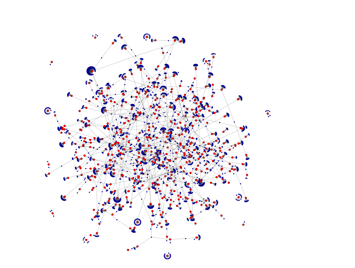
pgRouting, while designed for GIS route mapping, offers many functions that provide general graph-structure traversal. This allows us to play 'Six Degrees of Michael McDonald', where we see if we can link any two artists within a set cost. Or to visualize our entire graph. I'm using a (relatively) simple D3 force graph to create the visuals below. Feel free to rehost and play around.
.png)
What happened here? Well we have a a lot of multi-intersection nodes. Remember our artist count above? Jeff Porcaro performed on 90 songs, that's 90 lines exiting one node, and we can assume multiple artists performed on each song he performed, so that's going to create a very complicated network, with a lot of duplicate paths.
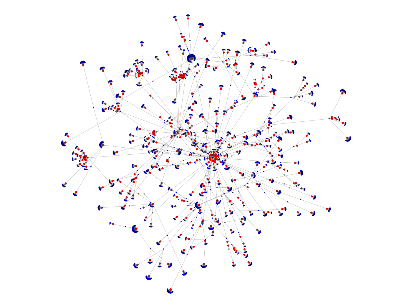
Let's simplify that and find our minimal spanning tree.
Our minimal network looks a lot less dense. It removes the clutter of repeated links (lines) while preserving all of the same nodes (dots).
This query represents the shortest paths that include every node in our graph. Each link or edge has a distance cost associated with it (remember, the smaller the better), which is used to generate the ‘cheapest’ (or in our case, yachtiest) network possible. The specific function used here is (pgr_kruskal)
select * from pgr_kruskal('select id, source, target, cost from node_map order by id');
Our minimal spanning tree returns 3848 out of 17758 edges. But, because our node_map includes mappings for both directions (source-> target and target to source), we know that that’s actually 3848 out of 8879 unique edges. That means there are around 5000 relationships that are 'not necessary' to complete our graph. They represent alternate connections between nodes, that's unsurprising when you consider that band members perform together on the same song, and don't need to be repeated for each connection.
So, where's Michael McDonald fit into all of this?
Right in the middle.
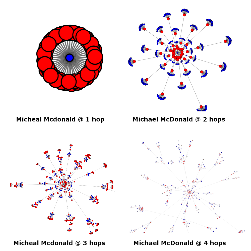
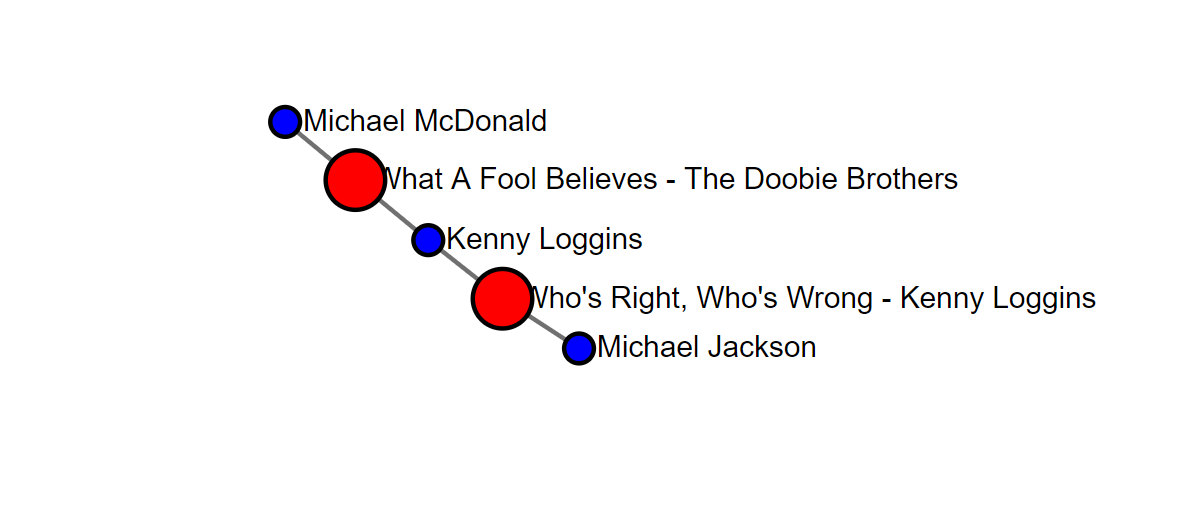
Our visualization above is built around the (pgr_drivingdistance) function. It travels our node map radiating from the provided starting id returning all paths that are less than or equal to our total cost distance. That looks like this:
select * from pgr_drivingdistance('select id, source, target 1 as cost from node_map', (select id from nodes where node_name = 'Michael McDonald'), 4);
By replacing our previously variable cost with static '1' we can count 'hops’ instead of distance. Each hop represents one edge, or one source -> target. By searching for a total cost of ‘1’, we can find all the songs McDonald performed on. If we look for a total cost of '2' we can find all the artists that performed on a song with McDonald. A total cost of '3' returns all the songs such that Michael McDonald -> song -> performer -> song. . . and so on.
Interestingly, our data will always alternate song -> performer (i.e. there's no artist -> artist relationship), and will always end on people on even hops and songs on odd hops. Our image above also shows a simple representation of the growth pattern at each hop. We can count our nodes at each step to produce the below table.
 hop  | count
------+-------
 1st  |    48
 2nd  |   502
 3rd  |   833
 4th  |  3364
 5th  |  3397
 6th  |  3723
 7th  |  3725
 8th  |  3737
 9th  |  3737
 10th |  3737
Each hop's node count includes the nodes in the previous hop. To get an accurate count, we need to subtract the previous hop's count to know how many new records were added. McDonald was on 47 songs. Those 47 songs had 474 artists, who in turn performed on 331 songs, which in turn had 2,481 new performers . . . and so on.
Our pattern is interesting, it bottlenecks on songs (there are less songs than performers). It also grows quickly at first but tapers off after the 4th step (because we have a finite non-evenly distributed data set, the fringes are harder to reach). We also can tell that we reach our full network size at the 8th hop. Since 8,9, and 10 are all equal, there's no growth, it’s the fullest representation of that portion of the Yacht Rock network.
So maybe we can use that to find who the yachtiest of the yachty is? Who 'completes' their network in the least number of hops?
We can create a function that finds the first hop where the count repeats for each performer.
CREATE OR REPLACE FUNCTION
    yre_get_complete_step(IN name_in text, OUT name text, OUT hop int, OUT nodes int)
AS $_$


DECLARE
    hop_c         integer := 1;
    old_nodes   integer := 0;
BEGIN


LOOP
    select name_in, hop_c, count(*)
      INTO name, hop, nodes
      from pgr_drivingdistance('select id, source, target, 1 as cost from node_map'::text,
            (select id from nodes where node_name = name_in), hop_c);

    IF nodes = old_nodes THEN
        hop = hop - 1;
        EXIT;
    ELSE
        hop_c := hop_c + 1;
        old_nodes := nodes;
    END IF;
END LOOP;

END;
$_$ LANGUAGE 'plpgsql';
And then populate a table with this information.
create table yacht_hops as (with n as (select node_name from nodes where node_type = 'performer') select y.* from n,yre_get_complete_step(n.node_name) as y);
On hour later, we have a table of every performer and how many hops it takes to reach every node in their network.
 nodes | count
-------+-------
  3737 |  3324
    18 |    34
    25 |    24
    15 |    14
    13 |    12
     7 |    12
     3 |     8
     4 |     6
     2 |     2
This helps us to define our disjointed networks. We can see here that we have different networks that aren't connected, at least 9 of them to be exact. We’ll refer to the largest noded network as the Yacht Rock core, and continue investigating there to find the center of the Yacht Rock universe. One might even question if those separated networks should even be considered part of the extended Yacht Rock universe. A deeper look into our core network shows something surprising.
select hop, count(*) from yacht_hops where nodes = 3737 group by hop order by hop asc;
hop | count
-----+-------
   6 |     2
   7 |     5
   8 |  1732
   9 |   159
  10 |  1369
  12 |    57
We have 5 artists that are able to traverse our core network in 7 hops, and 2 artists that can do it in 6. More surprisingly, McDonald isn't even in that list.
select name, hop, avg(cost) average, count(*) from yacht_hops yh join nodes n on yh.name = n.node_name join node_map nm on n.id = nm.target where hop in (6,7) and nodes =3737 group by name, hop order by hop,average,count;
      name      | hop |       average       | count
----------------+-----+---------------------+-------
 Jerry Hey      |   6 | 26.1302816901408451 |    71
 Nathan East    |   6 | 32.5517241379310345 |    29
 Steve Lukather |   7 | 24.7619178082191781 |    73
 Lenny Castro   |   7 | 26.2953846153846154 |    39
 Chuck Findley  |   7 | 26.8611111111111111 |    45
 Jeff Porcaro   |   7 | 27.4124444444444444 |    90
 Dean Parks     |   7 | 31.6293103448275862 |    29
I'm personally floored. No McDonald? No Cross! No Loggins! All Toto! All of the 'most connected' Yachters are Toto members, with the exception of Dean Parks, a studio musician with a bunch of Steely Dan appearances (7 of his 29 -- which places him pretty McDonald adjacent). sigh It's time to back off our original hypothesis and admit that Michael McDonald may not be at the helm of this ship.
Using our (in no way) entirely objective measuring criteria, I'd moor our ship to either Jerry Hey or Steve Lukather, and in a coin flip I'd pick Lukather -- he has a lower score (remember, lower is better here), and more name recognition to the average bosun. For the sake of completeness, here's What Lukather and Hey's graphs look like for the first four hops.
And while we didn't prove what we originally set out to, we did have a fun time getting here. We also just barely skimmed the surface of both pgRouting and Yacht Rock.
We could have looked at routing maps:
select * from pgr_dijkstra('select id, source, target, cost from node_map',
	(select id from nodes where node_name = source_name_in),
      (select id from nodes where node_name = target_name_in))
Or we could have looked at our Yacht scores differently by generating output from an All Pairs query (warning, this takes as long as you think it would . . .my query still hasn't returned hours later).
select * from pgr_floydwarshall('select id, source, target, cost from node_map');
The key is that pgRouting doesn't need to be limited to just routing spatial data, the general node-edge structure allows for many types of analysis. The data and visualization points are hosted athttps://www.yachtrockexplorer.com and https://github.com/scurvyjtp/yachtrockexplorer.
The ocean is your bounty, let Yacht Rock be your soundtrack.
